Margin Requirements Across Equity-Related Instruments: How Level Is the Playing Field?

Peter Fortune

The author is Senior Economist and

Advisor to the Director of Research at

the Federal Reserve Bank of Boston. He

is grateful to Michelle Barnes, Jeffrey

Fuhrer, and Richard Kopcke for con-

structive comments.

Margin Requirements

Across Equity-Related

Instruments: How Level

Is the Playing Field?

hen interest rates rose sharply in 1994, a number of derivatives-

related failures occurred, prominent among them the bankrupt-

cy of Orange County, California, which had invested heavily in

structured notes called “inverse floaters.”

These events led to vigorous

public discussion about the links between derivative securities and finan-

cial stability, as well as about the potential role of new regulation. In an

effort to clarify the issues, the Federal Reserve Bank of Boston sponsored

an educational forum in which the risks and risk management of deriva-

tive securities were discussed by a range of interested parties: academics;

lawmakers and regulators; experts from nonfinancial corporations,

investment and commercial banks, and pension funds; and issuers of

securities. The Bank published a summary of the presentations in

Minehan and Simons (1995).

In the keynote address, Harvard Business School Professor Jay Light

noted that there are at least 11 ways that investors can participate in the

returns on the Standard and Poor’s 500 composite index (see Box 1).

Professor Light pointed out that these alternatives exist because they dif-

fer in a variety of important respects: Some carry higher transaction costs;

others might have higher margin requirements; still others might differ in

tax treatment or in regulatory restraints.

The purpose of the present study is to assess one dimension of those

differences—margin requirements. The adoption of different margin

requirements for otherwise identical risk and reward positions might cre-

ate an uneven playing field that shifts traders and investors from high-

margin to low-margin instruments as they seek greater leverage or lower

carrying costs. This can result in inefficient trading, as when traders pay

Fortune pgs 31-50 1/6/04 8:21 PM Page 31

32 2003 Issue New England Economic Review

higher trading costs in order to gain the benefit of

lower margin requirements, and it can reduce the abil-

ity of financial agents to distribute risks in a way that

minimizes financial volatility.

This study focuses on equity-related instruments:

stocks, stock index instruments, stock options, stock

index options, futures on stocks and stock indexes,

and options on those futures. Section I provides back-

ground on these financial instruments and on the mar-

kets in which they are traded. Section II demonstrates

that, in the absence of margin requirements, strategies

using options, futures, and options on futures can

duplicate the returns on a leveraged purchase of

stocks or a stock index. Though these strategies are

shown to be identical in their risks and returns, differ-

ences in margin requirements might create incentives

to prefer one strategy over others.

Section III provides a background for understand-

ing margin requirements in stocks, options, futures,

and futures options. This is essential to the modeling

of margin requirements on each of the replicating port-

folios discussed in Section II. Section IV develops a

model to simulate the values arising from several

identical positions obtained by combinations of stocks

and stock derivatives. The results are then used to

assess, for each of the strategies identified in Section II,

the costs of margin requirements. This allows judg-

ments about the relative effects of differential margin

requirements.

Our primary conclusion is that the playing field

is more level than a cursory focus on initial margin

requirements might indicate. We find that the costs

associated with margin requirements on equities or

stock indexes—costs embedded in the Federal

Reserve Board’s Regulation T—are essentially fixed

costs: Only in the event of extreme price declines

do maintenance margin calls occur; Regulation T’s

initial margins are typically the sole source of mar-

gin-related trading cost. On the other hand, costs of

margin requirements on derivatives, particularly on

futures contracts, have a low fixed cost component

but are more sensitive to the price of the underlying

security: While maintenance margins on equities

rarely come into play, the practice of requiring varia-

tion margin on derivatives induces highly variable

costs.

Box 1

Eleven Ways to Buy the S&P 500 Index

• Purchase every one of the 500 stocks in the index;

• Buy one of a number of futures contracts trading

on the S&P 500;

• Negotiate a forward contract on the index with a

private intermediary, such as an investment bank;

• Buy a call option on the S&P 500, which would

allow one to capture the capital gains on the S&P

500, should prices rise;

• Buy the 500 stocks in the index and a put option,

yielding the same result as buying a call option,

namely, ensuring against a drop in the price of the

index while allowing one to benefit from a rise in

its price;

• Buy a bond convertible into the S&P 500 at face

value;

• Buy from a Wall Street dealer a structured note

with an interest rate tied to the return on the S&P 500;

• Buy from a bank an equity-linked Certificate of

Deposit that would pay a guaranteed minimum

rate, but if the S&P 500 increased over a certain

level, the interest rate would be tied to that increase;

• Buy a Guaranteed Investment Contract with the

same linkage from a life insurance company;

• Enter into an equity swap where one would pay a

floating interest rate (usually the London Interbank

Offered Rate, known as LIBOR) and receive the rate

of return on the S&P 500; or

• Buy a unit investment trust that holds the S&P

500; an example is a SPDR, traded on the American

Stock Exchange.

Source: Professor Jay Light, as quoted in Minehan and Simons

(1995), p. 6.

These notes paid an interest rate that fell when the general

level of interest rates increased, exposing the county to revenue

shortfalls that threatened its ability to meet its obligations, as well as

to capital losses on the notes.

Fortune pgs 31-50 1/6/04 8:21 PM Page 32

2003 Issue New England Economic Review 33

In short, players in the different markets might

not select their instruments on the basis of initial mar-

gins, and the differences in average costs, though sig-

nificant, might not be the primary reason to choose

one instrument over others. Rather, investors and

traders might be motivated by a choice between fixed

and variable margin costs: Risk-tolerant investors

choose instruments with high variable and low fixed

costs, such as futures or options, while less risk-toler-

ant investors select instruments with low variable but

high fixed costs. Rather than the playing field being

uneven, each instrument might be traded on a differ-

ent playing field.

Caveats are in order. This study does not address

the effects of other factors affecting an investor’s deci-

sion about which markets to use to achieve a path of

financial returns; among these other factors are com-

missions and fees, taxes, and regulatory or legal

restrictions. It is also based on a small subset of equity-

related instruments traded on registered exchanges;

over-the-counter (OTC) instruments, which have no

standardized margin-related costs, are not considered.

Finally, the analysis is based on simulations of prices

following standard pricing models with random

return-generating processes. While this incorporates

known aspects of the probability distribution of

returns on common stocks, the results cannot be gen-

eralized to specific portfolios in specific periods, nor

can they be applied to conditions of extreme financial

duress, during which probability distributions might

be different from the norm.

I. Equity-Related Financial Instruments

According to Ritchken (1987), organized trading

in stock options began in London in the eighteenth

century. By the late eighteenth century, option trading

had spread to the United States. Though tainted by

abuses, such as investors granting call options to bro-

kers who would recommend their stocks, the market

remained unregulated until the broad securities regu-

lation of the 1930s. Among the important legislative

actions was the Securities Exchange Act of 1934 (Act of

1934), which formed the Securities and Exchange

Commission (SEC) and authorized it to oversee

exchanges and broker-dealers trading stock and stock

options. The Act of 1934 also gave the Federal Reserve

Board the authority to set margin requirements on a

broad range of financial instruments.

Prior to 1973, the market for put and call options

on common stocks was an OTC market conducted by

dealers belonging to the Put and Call Dealers

Association. Because options contracts were written

directly between buyer and seller, counterparty risk

(the risk that the other party would fail to perform)

was high. And because the contracts were not stan-

dardized, they were illiquid and not easily resold. To

remedy these problems, the Chicago Board Options

Exchange (CBOE) was formed in 1973 to trade equity

options (options on individual stocks). The CBOE pro-

vided standardized contracts and established a clear-

inghouse that guaranteed the performance of con-

tracts, thereby shifting the counterparty risk from the

buyer and seller to clearinghouse members. These

innovations mitigated counterparty risk and enhanced

liquidity by allowing exchange-traded options posi-

tions to be easily reversed by offsetting trades: A hold-

er (writer) of a standardized call option could sell

(buy) an identical call option, thereby neutralizing his

position. The counterparty risk taken by the CBOE

clearinghouse led it to establish initial and mainte-

nance margin requirements to protect itself from fail-

ure of its clearing members.

In 1982, the CBOE initiated trading in put and call

options on the S&P 100 stock index option, the first

stock index option traded in the United States. In 1993,

the CBOE began trading S&P 500 Depository Receipts

(“Spiders”), the first Exchange Traded Fund (ETF),

and options on Spiders. A popular way to mimic the

S&P 500 index, Spiders differ from open-end mutual

funds, such as Vanguard’s S&P 500 Index Fund, in sev-

eral important ways: They (and other ETFs) are traded

continuously throughout the day, they can be sold

short, and they can sell at a premium or discount to net

asset value.

Both equity options and options on ETFs, which

trade like stocks, are American-style, meaning that

they can be exercised at any time up to the expiration

date. Stock index options are typically European-

style, so they can be exercised only on their expira-

tion day. For example, both European-style S&P 500

stock index options and American-style ETF options

on Spiders are currently traded. Each S&P 500 stock

index option contract (and each Spider option) is for

100 units of the S&P 500, and it expires on the third

Friday of the delivery month. On June 13, 2003, the

CBOE’s S&P 500 stock index option contracts traded

with delivery months of June, September, December,

and March. Strike prices ranged from 500 to 1700. At

The premium or discount is kept small by arbitrage. If, say, a

discount emerges, a trader can buy the S&P 500 stocks and convert

them into Spiders, thereby increasing the price of the underlying

stocks and reducing the price of the Spiders.

Fortune pgs 31-50 1/6/04 8:21 PM Page 33

34 2003 Issue New England Economic Review

the close of trading, the S&P 500 index was 988.61,

and the premium on the 995 September call option

was $35.00. Thus, one contract could be purchased

for $3,500 (= 100 times $35.00). If, say, the S&P 500

index closed at 1015 on the third Friday of

September, the holder of a Spider call option could

pay $99,500 (= 100 times $995) to take delivery of 100

units of S&P 500 worth $101,500 (= 100 times $1,015).

The sum of the gain on the option ($2,000) less the

premium paid ($3,500) yields a net loss of $1,500. The

loss, while regrettable, is smaller than the loss that

would have been experienced if the options had

expired unexercised.

Like options, forward contracts have existed in

the commodities markets for centuries. Forward con-

tracts are customized OTC agreements between two

parties. Like OTC options, they are not standardized,

are difficult to resell, and can carry significant counter-

party risk. The introduction of stock index futures con-

tracts in 1982 was an innovation on a par with the

development of exchange-traded equity and stock

index options. Unlike forward contracts, stock index

futures contracts are standardized instruments, traded

on organized exchanges and cleared through clearing-

houses that guarantee performance. Futures contracts

have less counterparty risk because of the clearing-

house guarantee, and, unlike forward contracts, which

typically involve no payments until they are exercised,

futures contracts require regular collection of “varia-

tion” margin to protect the clearinghouse. Stock index

futures contracts are now traded on the Chicago

Mercantile Exchange (CME), the Chicago Board of

Trade (CBOT), the Kansas City Board of Trade

(KCBOT), and the New York Financial Exchange

(NYFE).

Until recently, futures and futures options on indi-

vidual stocks (so-called “single-stock” futures) were

prohibited. In November 2002, after two years of dis-

cussion, single-stock futures began trading on two

exchanges: OneChicago, a joint venture of the CME,

CBOT, and CBOE; and Nasdaq-LIFFE, a joint venture

of Nasdaq and the London International Financial

Futures and Options Exchange (LIFFE). Nasdaq-LIFFE

initiated trading of futures on ten individual stocks

and on four ETFs.

OneChicago began by trading in

futures on 21 individual stocks, four of which were

also traded on Nasdaq-LIFFE.

A futures contract requires the seller to deliver the

underlying instrument at the futures price set at the

time of the contract. For example, one Russell 2000

contract traded on the CME has a notional value of

$500 times the Russell 2000 index; at the June 13 clos-

ing index of 449.71, the notional value of one contract

was, therefore, $224,855. The June 13 settlement price

(closing price) for the September contract, expiring on

the third Friday of September, was 450.75. Thus, the

buyer of one September contract at the June 13 settle-

ment price agreed to pay $225,375 (= 500 times

$450.75) to take delivery of 500 units of the Russell

2000 on the third Friday of September. If the Russell

2000 was higher than 450.75 on that date, say, at 455,

he would make a profit on the marked-up futures con-

tract, paying 450.75 for a contract worth 455; the profit

to the holder, and loss to the seller, would be $2,125 [=

500 x ($455 – $450.75)].

In 1982, the Commodities Futures Trading

Commission (CFTC) allowed exchanges to trade

options on any futures contract they traded.

Exercisable at any time before expiration, hence

American-style, an option on financial futures

involves delivery of one specific futures contract at the

exercise date. Options on futures expire at the same

time the underlying futures contract expires, the third

Friday of the futures delivery month. On June 13, 2003,

a 1040 September call option on the September S&P

500 futures contract had a premium of $16.70, or $4,175

per contract (= 250 times $16.70). If, say, at the end of

July, the call option had been exercised, the holder

would have paid $260,000 (= 250 x $1,040) for a

September S&P 500 futures contract. If the S&P 500 at

that time had been 1050, the futures contract received

would have been worth $262,500. The profit on the

option ($2,500) partly defrays the $4,175 premium

paid for the option, leaving a net cost of $1,675. If the

futures contract is held after it is delivered, there are

additional gains or losses as the contract is marked to

market each half-day.

Contracts on stock and stock index options have

been regulated by the SEC since its formation under

the Act of 1934. After the Commodities Futures

Trading Commission Act created the CFTC in 1974,

a number of jurisdictional disputes arose between

the SEC and the CFTC. These culminated in a 1981

agreement that the SEC would continue to regulate

cash market products, like equity and stock index

options, while futures and options on futures would

be regulated by the CFTC. That agreement is still

in effect.

The ten individual stocks were Chevron Texaco, Exxon

Mobil, Ford Motor, General Electric, General Motors, Honeywell,

IBM, Intel, Microsoft, and Oracle. The four ETFs were the Nasdaq-

100 tracking stock and contracts on the Russell 1000, Russell 2000,

and Russell 3000 stock indexes.

Fortune pgs 31-50 1/6/04 8:21 PM Page 34

2003 Issue New England Economic Review 35

II. Derivative Instruments and Replicating

Portfolios

We now show that several strategies, called

“replicating portfolios,” can be designed using stocks

and their derivative securities. Each of these portfolios

uses different instruments to achieve identical risks

and returns. Each is constructed to be costless, requir-

ing no initial cash payments at the outset. Having

shown that there are several strategies to construct

portfolios with identical financial rewards and risks,

using cash instruments, futures instruments, or deriv-

atives, we next introduce margin requirements as a

cash obligation. We then consider the effects of these

requirements on the costs of each replicating portfolio.

Variables and formulas are denoted by bold-faced

type.

Consider an investor who structures a portfolio

that will be liquidated at future time T. She can invest

in common stock or a stock index, in a futures contract

on the stock or stock index, in a call or put option on a

futures contract on the stock or stock index, or in an

option on the stock or stock index. A purchase at price

S of common stock, of a stock index, or of an ETF can

be financed by a margin loan in amount D; this is a

“leveraged purchase of common stock.” Interest on the

margin loan, at rate r, accumulates until the debt is

repaid at time T. After T periods (“days”) have passed,

the value of the stock is S

, the margin loan repayment

is D(1+r)

, and S

– D(1+r)

is the profit or loss.

Suppose now that no margin is required: The investor

can borrow the full amount of the stock or stock index,

that is, D = S, and the fully leveraged purchase is said

to be “costless” because it requires no initial cash out-

lay. The terminal value of the fully leveraged purchase,

sans margin requirements, is S

– S(1+r)

This fully leveraged purchase can be replicated by

the use of European-style options on the same under-

lying security. Purchase of a call option with strike

price X at premium C, combined with simultaneous

sale of a put option with the same strike price at pre-

mium P, will have a profit of S

– [X + (C-P)(1+r)

] at

the end of T periods. The cost in brackets is the strike

price plus the accumulated value at T of the income

foregone from the initial net premium paid. The put-

call parity theorem, a well-known theorem of option

finance, states that the call and put premiums will be

equal when the option strike price is selected to be X =

S(1+r)

. For an option with this strike price, the option

strategy is costless (C = P), and the value at time T is

– S(1+r)

. This strategy has the same initial cash

outlay and terminal value as the leveraged purchase. It

is, therefore, a replicating portfolio, identical to the

leveraged purchase.

Yet another strategy that replicates the fully lever-

aged purchase (and the stock option strategy) is to buy

a futures contract that expires after T periods. The

futures price at the time the contract is made is F dol-

lars. Because a futures contract is an agreement to

make an exchange in the future, not a purchase or sale

requiring a cash outlay, the futures contract, excluding

margin requirements, is, like the fully leveraged stock

purchase, costless at the outset. After T periods, it will

be worth S

– F. But index arbitrage

by profit-seeking

arbitrageurs will ensure that the futures price will be

F = S(1+r)

, so the final value of the futures contract is

– S(1+r)

, identical to the value of the fully lever-

aged investment in common stock.

The final replicating portfolio we consider is pur-

chase of a futures call option with strike price X =

S(1+r)

, paying premium C, combined with simultane-

ous sale of a put option on the same futures contract at

the same strike price and at premium P; the initial cash

outlay is C-P, and the cost at T is (C-P)(1+r)

. Because

one of the options will be exercised—either the put or

the call will expire in the money—the value of this

combination will be F

at the expiration of the options.

This must be equal to the cash stock price, S

, at that

date, so the net profit will be S

– [X + (C-P)(1+r)

Setting the strike price at X = S(1+r)

, and invoking the

put-call parity theorem to ensure that C = P, the termi-

nal value is S

– S(1+r)

Once again, this is identical

to the value at T of the fully leveraged purchase.

Thus, financial theory suggests that with four

instruments (stock, futures, options on stocks, and

options on futures), there are four equivalent strate-

gies for achieving a final position equivalent to a lever-

aged purchase of common stocks. However, margin

requirements will create differences in the attractive-

ness of these replicating portfolios. Before explicitly

Investors can buy the stock in the cash market for S dollars.

The opportunity cost at time T will be S(1+r)

. Alternatively, they

can buy a futures contract for F dollars. Both will be worth S

at time

T, and each has the same risk arising from the stock’s price volatili-

ty. Thus, the equality F = S(1+r)

is the equilibrium relationship

between the futures and the cash price of the stock. If, for example,

the stock price is too low and the futures price too high, the first

investment (purchase stock) will be more profitable than the second

investment (purchase a futures contract), and investors will buy

stocks and sell futures contracts until the equality is restored.

If option holders exercise options early, the pricing relation-

ships on which our analysis rests will not be exact: An option that

can be exercised early might have a value greater than a European

option. However, this possibility is not likely to dramatically alter

our results. Early exercise of options is typically associated with

options that are deep in-the-money or for which the underlying

asset pays a cash dividend at specific intervals.

Fortune pgs 31-50 1/6/04 8:21 PM Page 35

36 2003 Issue New England Economic Review

modeling the effect of margin requirements, we review

their nature and history.

III. Margin Requirements for Equity-Related

Securities

The function of a “margin requirement” varies

according to the security bought or held. In equity

markets, where broker-dealers or other financial insti-

tutions lend money to customers for purchasing or

holding common stocks, margin requirements rest on

four philosophical legs. The first, lender protection, is to

ensure that the broker-dealer’s loan is repaid, mitigat-

ing systemic problems arising from broker-dealer fail-

ures. The second, investor protection, is to limit the abil-

ity of investors or traders to expose themselves to

excessive risk through the leverage allowed by bor-

rowed funds. The third, market protection, is to enhance

market stability by providing an equity cushion that

reduces the probability of margin calls, mitigating

forced sales in times of falling prices, and raises the

cash cost of purchasing stocks, inhibiting overly opti-

mistic buyers in times of rising prices. The fourth, cred-

it allocation, arises from a concern about the potential

diversion of credit from legitimate business uses to

speculative activity.

But for derivative securities there is no explicit

loan to be protected. Furthermore, protecting investors

from themselves and enhancing stability of the market

for the underlying security are distinctly secondary

considerations. Rather, as noted above, the primary

purpose of margin requirements on derivatives is to

provide a performance bond, protecting each party

from the costs of the counterparty’s failure to complete

the contractual obligation. For example, the writer

(seller) of a call option on common stock has the obli-

gation to deliver the specified number of shares (typi-

cally 100 shares per option contract) if the buyer exer-

cises the option. Should the writer fail to deliver on

time, the buyer will have overpaid for the option and

will not receive the benefit of the hedging or other

strategy that motivated the purchase.

Margin requirements have several key character-

istics: (1) the initial margin, the minimum equity

required at the time a position is taken; (2) the mainte-

nance margin, the minimum equity to be maintained

during the time a position is open; (3) the variation mar-

gin, the additional margin required, or release of mar-

gin allowed, as prices of underlying securities change;

(4) the settlement period, the interval between times

when the value of the account is updated and calls for

additional margin are issued; (5) the payment period,

the time allowed for initial or additional margin to be

posted to the account; and (6) the acceptable collateral,

the collateral that can be used to meet initial or mainte-

nance margin calls. We consider each of these charac-

teristics in the equity, options, and futures markets.

Our focus is on the rules that apply in the New York

Stock Exchange (NYSE), the Chicago Board Options

Exchange (CBOE), and the Chicago Mercantile

Exchange (CME). Standards set at other exchanges

typically mirror standards at these major exchanges.

Minimum margin requirements set by the exchanges

are subject to approval by the appropriate regulatory

agency—the Securities and Exchange Commission for

stocks and stock options, and the Commodities

Futures Trading Commission for futures and futures

options.

A distinction is often made between “strategy-

based” and “portfolio-based” margin systems.

Strategy-based margin systems consist of fixed rules,

often independent of the precise characteristics of an

account, such as its volatility or asset structure. To the

extent that strategy-based systems recognize combina-

tions of securities, they do so by applying fixed rules

for “offsets” in defined combinations. Thus,

Regulation T’s requirement that the margin be no less

than 50 percent of the value of common stock is strate-

gy-based, as is the CBOE’s rule that the margin

required of a covered call option be equal to 50 percent

of the value of the underlying stock. Strategy-based

margin systems are typically set at the federal or

exchange levels.

Portfolio-based margin systems set margin

requirements by simulating the value of the account

over a pre-set interval of time, using the asset alloca-

tion, volatility, and price characteristics specific to the

customer’s account. Margin requirements are then set

to avoid all but worst-case outcomes. Portfolio-based

margin systems are typically used by broker-dealers

and clearinghouses. Regulatory agencies are in the

process of reducing reliance on strategy-based systems

and focusing their efforts on evaluation and monitor-

ing of portfolio-based systems implemented by

exchanges and clearinghouses. We will discuss portfo-

lio-based margining below, when we address margin

requirements at clearinghouses.

Margin Requirements for Common Stocks

Margin requirements for common stocks are set at

three levels. First, “federal margin requirements” are

embodied in the Federal Reserve System’s Regulation

Fortune pgs 31-50 1/6/04 8:21 PM Page 36

2003 Issue New England Economic Review 37

T, for broker-dealer loans, and Regulation U, for loans

by bank and nonbank institutions. These regulations

have been discussed recently in this Review (Fortune

2000 and 2002). Regulation T specifies those stocks and

equity-related instruments that are marginable, that is,

that have loan value, and it sets their margin require-

ments. The current margin requirements are shown in

Table 1.

An investor purchasing, say, $100,000 of common

stock, can borrow no more than 50 percent of the pur-

chase price, or $50,000; the equity (or “margin”)

required is, therefore, $50,000. The investor who sells

$100,000 of common stock short must place the pro-

ceeds with the lender of the stock as collateral and

must also have equity of $50,000 in his account. Thus,

the effective margin for a short seller is 150 percent of

the initial value of the position.

The purpose of the

margin for a loan to buy stock is to protect the broker

as a lender of cash; the purpose in a short sale is to pro-

tect the broker as a lender of securities.

Regulation T requires that initial margin be post-

ed within one “payment period” of the trade, defined

as the number of business days in the “standard settle-

ment cycle” plus two days. Because the standard set-

tlement for common stocks is three days, the payment

period for common stocks is five days. Initial margin

can be in the form of cash, exempt securities (such as

U.S. Treasury or municipal bonds), margin securities,

or a transfer from the Special Memorandum Account,

or SMA (see Fortune 2000).

Only the loan value of a

margin security can be used to meet margin calls, so if

an investor wants to deposit, say, $10,000 in shares of

margin stock to meet a federal margin call, only 50 per-

cent, or $5,000, can be used to meet the call.

Under Regulation T, the Federal Reserve Board

has the authority to set maintenance margin require-

ments for equities. However, the Board has delegated

this authority to the exchanges on which the stocks are

traded, subject to the SEC’s approval of the exchange

as a Self Regulatory Organization (SRO). Positions in

margin accounts are marked to the market at the end

of each day, at which time calculations for federal mar-

gin excess or deficiency are made: A federal margin

deficiency arises when the account’s margin is less

than the margin required by Regulation T. No federal

margin calls are issued if a federal margin deficiency

exists, but margin-deficient accounts are “restricted”

until the margin is restored to the initial level required

by Regulation T.

Table 1

Margin Requirements for Single-Equity Securities

Margin Margin

Security Type Exchange (Speculator) (Hedger, et al.)

Main- Main-

Initial tenance Initial tenance

Single Stocks New York Stock Exchange 50%

25%

50%

25%

American Stock Exchange 50%

25%

50%

25%

Nasdaq 50%

25%

50%

25%

Single Stock American Stock Exchange See Table 2 See Table 2 See Table 2 See Table 2

Options (AMEX, CBOE)

Single Stock OneChicago 20%

20%

Futures (CME)

Nasdaq-LIFFE

(NQLX)

Source: Federal Reserve System, New York Stock Exchange, Chicago Board Options Exchange, OneChicago, Nasdaq-LIFFE, Chicago Mercantile

Exchange, Wall Street Journal.

Percent of value, Board of Governors of the Federal Reserve System, Regulation T.

Percent of value, New York Stock Exchange, American Stock Exchange, and Nasdaq.

Percent of value, OneChicago (joint venture of Chicago Mercantile Exchange, Chicago Board of Trade, and Chicago Board Options Exchange).

Brokers typically require collateral of 102 percent of the value

of securities they lend, thus raising the effective margin required for

a common stock short sale to 152 percent.

The SMA is a margin account’s record of cash deposits and of

transfers of excess margin from the margin account. With some

restrictions, SMA balances can be used to satisfy margin calls.

Owners of restricted accounts cannot withdraw funds or sub-

stitute securities if this would further increase the margin deficiency.

Fortune pgs 31-50 1/6/04 8:21 PM Page 37

38 2003 Issue New England Economic Review

The exchanges on which the stock is traded set

“exchange” margin requirements.

Currently, the

exchange margin requirements for common stock

traded on the New York Stock Exchange, the American

Stock Exchange, and Nasdaq are uniform: NYSE Rule

431 and NASD Rule 2520 require maintenance margin

of at least 25 percent of the value of stock held long

and 30 percent of the value of stock sold short. Specific

hedged positions are subject to different requirements.

For example, stocks sold short against the box (a long

position offset by a short position) must maintain mar-

gin equal to 5 percent of the long position. The settle-

ment period for exchange margins is daily, that is, the

value of, and margin in, an account are computed at

the close of trading, and any margin calls are immedi-

ately issued. Rule 431 requires satisfaction of exchange

margin calls within 15 days. The collateral allowed by

NYSE is that allowed by Regulation T: Margin calls

can be satisfied by deposit of cash, exempted securi-

ties, or margin securities, or by a transfer from the

SMA. Again, only the loan value of securities can be

used to meet a margin call. For example, with an

exchange margin of 25 percent, only 75 percent of the

deposit of margin stock can be used to meet an

exchange margin call.

Brokers also set “house” margin requirements

using portfolio-based margin systems. House margins

can be no lower, and are often higher, than exchange

margin requirements. Recent indications suggest that

house margin requirements have typically been 35

percent of the value of margin securities, although

during the stock market bubble of the late 1990s some

brokers set house margin requirements on specific

classes of stock as high as 100 percent (no loan value).

While stock exchange rules require that margin calls

must be met within 15 days, brokers rarely allow that

much time: House margin calls are rarely outstanding

for more than five business days,

and brokers can

require immediate payment or unilaterally liquidate

under-margined positions at their discretion. Variation

margin is not mandated by federal, exchange, or house

margin requirements. Thus, daily price fluctuations do

not give rise to margin calls unless the margin falls

below the level required by the house or by the

exchange.

Transactions in common stocks and many other

securities are cleared through the Depository Trust

and Clearing Corporation (DTCC), created by a recent

merger of the National Security Clearing Corporation

(NSCC), which provided clearing and settlement serv-

ices, and the Depository Trust Corporation (DTC),

which maintains the electronic registry of stock owner-

ship. While DTCC has membership criteria and uses

capital standards and other methods of ensuring that

its members make the payments that transactions

require, it does not set margin requirements for com-

mon stocks.

Margin Requirements for Equity or

Equity Index Options

Once the terms of, and parties to, a trade are veri-

fied, the obligation to deliver and make payment for

option contracts is assumed by the clearinghouse. In

the case of exchange-traded equity options, all clearing

is done by the Options Clearing Corporation (OCC).

The OCC establishes margin requirements to ensure

that the risk it acquires from performance guarantees

is minimal.

The options exchanges establish both initial and

maintenance margin requirements, specify the pay-

ment period within which margin must be paid, and

dictate the instruments that are acceptable for satisfac-

tion of margin requirements. The CBOE’s Rule 12.2

follows the federal and exchange standards for com-

mon stock payment periods by specifying that initial

margin must be obtained as promptly as possible but

no later than five days after the trade, and that mainte-

nance margin must be obtained as promptly as possi-

ble but within 15 days of the margin deficiency. The

CBOE requires that option contracts be marked to

market daily: At the end of each trading day, margin

surplus or deficiency is calculated, and margin calls

are issued by 7:00 a.m. the following day. Margin calls

must be satisfied by 9:00 a.m. unless a waiver is grant-

ed. Margin can be paid in cash or in “cash equivalents”

as defined in Regulation T’s section 220.2: U.S.

Treasury securities, negotiable bank CDs, bankers

acceptances issued by U.S. banks and payable in the

United States, and money market mutual funds.

Table 2 shows the CBOE’s minimum margin

requirements for naked options—options that are not

used as hedges or in combination with other options—

as well as for several option spreads and combina-

tions. For example, under CBOE Rule 12.3, the buyer

of a CBOE-listed option less than nine months to expi-

Exchanges also have the authority to set initial margin

requirements if they do not violate the requirements of Regulation T.

This authority is rarely used, although there are some prominent

examples of exchanges setting 100 percent initial margins for some

highly volatile stocks.

The SEC’s Rule 15c3-1 requires a charge against a broker-

dealer’s net capital for margin calls outstanding for more than five

days. This discourages brokers from extending calls beyond that

time.

Fortune pgs 31-50 1/6/04 8:21 PM Page 38

2003 Issue New England Economic Review 39

ration must pay in full, and the seller (writer) of a

naked equity option must satisfy an initial margin

requirement equal to the option sale’s proceeds plus

the greater of (a) 10 percent of the value of the under-

lying securities, or (b) 20 percent of the value of the

underlying security less the amount by which the con-

tract is out-of-the-money.

The initial margin require-

ment formula must be maintained throughout the life

of the contract; hence all gains and losses give rise to

variation margin so that, for example, the naked call

option writer must maintain margin equal to the

option’s premium plus the greater of (a) 10 percent of

the underlying security value, or (b) 20 percent of

the underlying security value less the amount out-of-

the-money.

Options written in combination with other

options or underlying securities have lower margin

Table 2

Margin Requirements for Listed Equity-Related Options

Chicago Board Options Exchange

Underlying

Position Security Margin Requirement

Naked Option: Equity Initial: 100% of premium (75% if expiration > 9 months)

Long Put or Long Call Broad Index Maintenance: None

Narrow Index

Naked Option: Broad Index Initial: 100% of premium + 15% of underlying value (if broad index) or 20% of

Short Put or Short Call Narrow Index underlying value (if equity or narrow index) – amount out of the money

(any expiration) Equity Maintenance: Equal to initial

Covered Call: Broad Index Initial: No requirement on short call; 50% on long stock (Reg T)

Short Call + Long Stock Narrow Index Maintenance: No requirement on short call; 25% on long stock (NYSE)

Equity

Long Straddle: Broad Index Initial: 100% (75% if > 9 months) of premiums on both options

Long Put and Long Call

Narrow Index Maintenance: None

(equal strike prices) Equity

Short Straddle: Broad Index Initial: Greater of short put or short call requirement + 100% of premium

Short Put and Short Call

Narrow Index on other side

(equal strike prices) Equity Maintenance: Equal to initial

If short option expires at or before long option:

Initial: long paid in full (short proceeds can apply) + (1) difference between

Call Spread: long call and short call strikes, if positive; or (2) difference between

Long Call + Short Call Broad Index short put and long put strikes, if positive

Narrow Index

Put Spread: Equity

Long Put + Short Put If short option expires after long option:

Initial: long paid in full (short proceeds can apply) + margin required for

naked short option

Maintenance: Equal to initial

Collar: Equity Initial: Put premium + 50% of underlying value (Reg T)

Long Put + Short Call Broad Index Maintenance: Lower of (1) 25% of call strike, or (2) 10% of put strike + amount

+ Long Stock Narrow Index put is out of the money

(put strike < stock < call strike)

Source: Chicago Board Options Exchange Margin Manual, April 2000; Chicago Board Options Exchange Constitution and Rules, March 2001.

Minimum margin is option proceeds + (a) 10% of underlying security value if a call, or (b) 10% of strike price if a put.

If index, underlying index and index multiplier are same; if equity, same stock underlies both.

Applies if underlying security is the same for both options.

If the option written is a put, the requirement is sales pro-

ceeds plus the greater of (a) 10 percent of the strike price, or (b) 20

percent of the underlying value less the out-of-money amount.

Fortune pgs 31-50 1/6/04 8:21 PM Page 39

40 2003 Issue New England Economic Review

requirements. For example, writers of covered call

options, in which a call option is written while the

underlying stock is held, face only the Regulation T

and exchange requirements for the long stock position:

an initial margin of 50 percent of the value of the stock,

as set in Regulation T, and 25 percent of the value, as

set by the NYSE and other exchanges.

Margin in the Futures Markets

The CME and the CBOT have developed a com-

mon margin system for index futures and futures

options. As discussed above, until recently CFTC regu-

lations limited equity-related futures and futures

options to stock index contracts, such as the S&P 500.

In November 2002, trading in “single stock futures”

began. This includes trading in ETFs. Single stock

futures and futures options are traded on OneChicago,

a joint venture of CME, the CBOE, and the CBOT, or

on Nasdaq-LIFFE. The CME minimum margin

requirements are reported in Table 3. OneChicago’s

margin requirements for single stock contracts are

reported in Table 1.

Orders for futures and futures options are

processed through firms called Futures Commission

Merchants (FCMs), which act as the equivalent of

stock brokerage firms. Many FCMs are members of the

clearinghouse for the exchange on which they trade.

FCMs that are not clearing members must clear their

trades through a clearing member.

As in the options market, there is no explicit credit

risk, but each party faces the risk that the other party will

fail to deliver or accept delivery of the underlying secu-

rity. At the CME and CBOT, an initial margin require-

ment, called “original margin,” is set to assure perform-

ance. Original margin is higher for “speculators” than

for “other” customers (hedgers, specialists, and market

makers).

The New York Board of Trade (NYBOT), on

the other hand, does not currently have different

requirements for “speculators” than for “others.”

At the CME and CBOT, maintenance margin

requirements for both “speculators” and others are set

at the original margin required of others. Thus, specu-

lators’ excess original margins can be lost before main-

tenance margins come into play, while “others” must

meet margin calls for any losses. Maintenance margin

is obtained through collection of variation margin at

least twice a day. At the end of each day, an FCM’s

accounts are marked to market, and any gains or loss-

es since the previous mark-to-market are recorded. By

6:40 a.m. the following day these gains and losses are

reflected in calculations of “settlement variation,” after

which the CME instructs settlement banks to credit

gains to the FCM or to collect variation margin. At

11:15 a.m., positions are marked to market again, and a

mid-day variation margin is paid or collected at 2:00

p.m. Thus, margin positions are restored to the “other”

original margin level at least twice a day. Margin at the

“other” level is maintained at the exchange clearing-

houses, while the excess required of speculators is typ-

ically kept by the FCM. For example, for a futures con-

tract on the Russell 1000, the CME requires an original

margin of $4,250 for speculators and $3,400 for others.

The maintenance margin for both is set at the initial

“other” level ($3,400), and variation margin is collect-

ed at least twice a day to ensure that this is done. The

$3,400 maintenance margin is kept at the CME clear-

inghouse. If the trader is a speculator, the excess initial

margin, $850, is kept at the FCM.

In contrast to requirements for stocks, stock

options, and single-security futures, margin require-

ments for stock index futures are stated in absolute

dollars. Thus, the percent of margin required will vary

inversely with the stock index. For example, as noted

above, a contract on the Russell 1000 at the CME must

have original margin of $4,250 for speculators. If the

Russell 1000 index is 525, the notional value of a

futures contract is $262,500 ($500 times the index), and

the speculator’s original margin requirement is 1.6

percent of the value of a contract. But if the index rises

to 600, the margin required is 1.4 percent of the con-

tract value.

Clearinghouses collect margins from member

FCMs on either a gross margin or a net margin basis:

Gross margining is used at the CME, CBOT, and

NYBOT; net margining at other exchanges. Gross mar-

gin means that margin is collected on both short and

long positions; net margin means collection only on

net (long minus short) positions. For example, if a non-

speculator at an FCM is long 1000 S&P 500 futures con-

tracts, and another non-speculator at that FCM is short

900 S&P 500 contracts, the FCM’s net position is 100

long contracts, and its gross position is 1900 contracts.

At the minimum CME gross margin requirement of

$14,250 per S&P 500 contract, the FCM would collect

margin of $27,075,000 (= $14,250 x 1900). If net margin

is used, the margin deposited by the FCM would be

only $1,425,000.

There has been some debate over the possibility

that traders at exchanges using net margin systems are

The distinction among customers is similar to the practice in

the stock market, where Regulation T exempts market makers and

other specialists from the requirements that public customers face,

requiring only that lenders maintain “good faith” margins.

Fortune pgs 31-50 1/6/04 8:21 PM Page 40

2003 Issue New England Economic Review 41

advantaged relative to those at gross margin

exchanges. The argument is that traders will shift to

exchanges using net margin systems because smaller

clearinghouse margins are required. However, Rutz

(1989) discounts this, noting that commodities regula-

tions require FCMs to collect margins on gross posi-

tions.

Aclearinghouse using net margin does not

Table 3

Margin Requirements for Equity Index Securities

Security Traded Margin Margin

Security Type Exchange [Symbol or Multiple

] (Speculator) (“Other”)

Main- Main-

Initial tenance Initial tenance

Exchange Traded American Stock Exchange Dow Jones Indl [DIA] 50% 25% 50% 25%

Funds (AMEX) Nasdaq 100 [QQQ] 50% 25% 50% 25%

Russell 1000 (iShares) [IWB] 50% 25% 50% 25%

Russell 2000 (iShares) [IWM] 50% 25% 50% 25%

Russell 3000 (iShares) [IWV] 50% 25% 50% 25%

S&P 500 [SPY] 50% 25% 50% 25%

S&P 500 (iShares) [IVV] 50% 25% 50% 25%

Chicago Board Options Exchange Nasdaq 100 [QQQ] 50% 25% 50% 25%

(CBOE) S&P 100 (iShares) [OEF] 50% 25% 50% 25%

S&P 500 [SPY] 50% 25% 50% 25%

Index Options Chicago Board Options Exchange Dow Jones Indl [DJX] Table 2 Table 2 Table 2 Table 2

(CBOE) (broad) (broad) (broad) (broad)

Nasdaq 100 [NDX] “ “ “ “

Russell 2000 [RUT] “ “ “ “

S&P 100 [OEX, XEO] “ “ “ “

S&P 500 [SPX] “ “ “ “

Index Futures

Chicago Board of Trade Dow Jones Indl [$10 x Indx] $10,000 $10,000 $10,000 $10,000

(CBOT)

Chicago Mercantile Exchange Nasdaq 100 [$100 x Indx] $11,250 $ 9,000 $ 9,000 $ 9,000

(CME) Nikkei 225 [$ 5 x Indx] $ 6,250 $ 5,000 $ 5,000 $ 5,000

Russell 1000 [$500 x Indx] $ 4,250 $ 3,400 $ 3,400 $ 3,400

Russell 2000 [$500 x Indx] $15,000 $12,000 $12,000 $12,000

S&P 500 [$250 x Indx] $17,813 $14,250 $14,250 $14,250

New York Financial Exchange NYSE Comp [$500 x Indx] $10,000 $10,000 $10,000 $10,000

(NYFE) Russell 1000 [$500 x Indx] $10,000 $10,000 $10,000 $10,000

Index Futures Chicago Board of Trade Dow Jones Indl [$100 x Prem] Table 2 Table 2 Table 2 Table 2

Options (CBOT) (broad) (broad) (broad) (broad)

Chicago Mercantile Exchange Nasdaq 100 [$100 x Prem] “ “ “ “

(CME) Russell 1000 [$500 x Prem] “ “ “ “

Russell 2000 [$500 x Prem] “ “ “ “

S&P 500 [$250 x Prem] “ “ “ “

New York Financial Exchange NYSE Comp [$500 x Prem] “ “ “ “

(NYFE)

Source: Data obtained from each exchange.

For futures and futures options the contract value is determined by a multiple of the underlying stock index or the future option premium.

In September 2003, initial margins for index futures, as a percent of cash index level, were as follows: S&P 500: speculator = 6.9%, other = 5.5%;

Nasdaq: speculator = 8.1%, other = 6.5%; Russell 2000: speculator = 5.8%, other = 4.7%.

Section 1.58 of the Commodity Futures Trading Commission

Act of 1974, Title 17, Chapter 1, of the Code of Federal Regulations,

requires FCMs to collect exchange-required margin on “each position.”

Fortune pgs 31-50 1/6/04 8:21 PM Page 41

42 2003 Issue New England Economic Review

give its FCM customers an advantage because the cus-

tomer must have margin consistent with his gross

positions. The only effect is that the clearinghouse

holds the net margin, while the FCM holds the excess

of gross margin over net margin. In short, the distinc-

tion between net and gross margins at the clearing-

house affects only the division of the total margin

between the FCM and the clearinghouse.

Original margin requirements at the CME and

CBOT can be met in a variety of ways: cash (in several

currencies), U.S. Treasury securities, letters of credit

issued by approved banks, selected common stocks in

the S&P 500, sovereign Canadian bonds, discount

notes or noncallable bills of several federally support-

ed mortgage credit agencies, and certain money mar-

ket mutual funds. Variation margin must be paid

in cash through settlement banks accepted by the

clearinghouse.

Clearing House Margin

The Depository Trust and Clearing Corporation

(DTCC), the clearinghouse for common stocks, does not

set margin requirements because it does not loan

money to customers, nor does it have any obligation

after trades are cleared and settled. Once the trade is

cleared, the DTCC is no longer a party to any contract.

In contrast, clearinghouses at options, futures, and

futures-options markets incur counterparty risk from

the date a contract is initiated until the contract’s expi-

ration. The equivalent of a “house margin” is, therefore,

set by the clearinghouse associated with each exchange.

Clearinghouse margins are established using a

dynamic portfolio-margining model, rather than the

static, rules-based approaches used at the exchanges.

The clearinghouse for options, the Options Clearing

Corporation, uses a portfolio-based system called

Theoretical Intermarket Margin System (TIMS). The

clearinghouses for futures and futures options at the

CME, CBOT, NYBOT, OneChicago, and Nasdaq-

LIFFE use a similar portfolio-margin system, called

Standard Portfolio Analysis of Risk (SPAN).

The purpose of a portfolio-based margining sys-

tem is to provide estimates of the losses that might be

experienced on an account over the interval of time

that the clearinghouse allows for margin calls to be sat-

isfied. That interval is generally looser in the stock

market, where brokers can require immediate (intra-

day) payment but often give several days (rarely more

than five, but up to 15) for good customers.

Clearinghouses in the options, futures, and futures-

options markets have a weaker relationship with

traders because the clearing FCM puts them at one

degree of separation. Thus, clearinghouses are less

focused than brokerage firms on the business losses

that might ensue from aggressive margin collection.

As noted above, the OCC requires a daily margin set-

tlement in stock options, hence a one-day interval,

while the clearinghouse at the CME, where margin set-

tlement is twice daily, uses an interval of a half day.

An ideal portfolio margining system would gen-

erate a complete probability distribution of losses over

the selected interval. This would require information

on the joint probability distribution of the prices of all

underlying securities: All the relevant moments of the

distribution (mean returns, variances or “volatility,”

covariances, and higher moments) would be accurate-

ly measured and used. The characteristics of each

derivative security—its expiration date, convexity,

volatility, and so on—would be ascertained. Then the

returns for each account would be simulated, and mar-

gin would be set according to a loss criterion, such as

requiring margin to cover any losses up to those with a

probability of one percent or less.

The portfolio-margining systems currently in use

fall short of this ideal. Kupiec (1994) described and

simulated the SPAN system. The first step in SPAN is

to construct classes of stock index futures and index

futures option instruments based on the underlying

index. Prices of securities within each class are

assumed to be perfectly correlated, while across-class

correlations are treated as zero except in certain cir-

cumstances. For each class, the values of several risk

parameters are chosen, and a matrix of these parame-

ters for each security class is constructed. This “risk

array” is sent to each clearing member. The FCM then

uses the SPAN model and the common risk array to

calculate the potential value of each account’s gain or

loss over a one-day period.

The primary risk parameters used in SPAN are

the “futures-price scan range” and the “implied-

volatility scan range.” The futures-price scan range is

derived by using historical data to compute the range

of absolute changes in futures prices, assuming 95 and

99 percent confidence intervals and selected past win-

dow lengths (60 days, 120 days, and one year). The

precise futures-price scan range is then chosen from

these computations by the CME’s margin committee.

Because futures contracts have no convexity, the

futures-price scan range directly measures the gains or

losses on those contracts; therefore, it directly deter-

mines the margin requirement on a futures contract.

The convexity of futures options means that gains or

losses will depend on the initial prices as well as the

Fortune pgs 31-50 1/6/04 8:21 PM Page 42

2003 Issue New England Economic Review 43

price variability. The futures-price scan range is, there-

fore, an input to the risk array used with a futures-

option pricing model to compute margin requirements

for futures options.

The second parameter, the implied-volatility scan

range, is relevant to setting margin requirements for

futures options because, again as a result of convexity,

volatility is an essential input to option pricing. For

each index futures class, the implied volatility of the

underlying security is computed for nearest-quarter

expiration at several strike prices. An average of those

implied volatilities is computed, and then the frequen-

cy distributions of volatility changes for several time

windows are formed. The 95

and 99

percentile val-

ues of volatility changes are computed, and the

implied-volatility scan range is then chosen from these

by the margin committee.

Other risk parameters are the “calendar spread

charge,” which is an additional margin required to

reflect price volatility on futures options with different

expiration dates; the “short option charge,” which is

the minimum margin requirement for a short option;

and the “inter-commodity spread charge,” which

reflects ad hoc judgments about

correlations across instruments.

SPAN calculations are done

for a pre-set list of 16 scenarios,

each differing in the combina-

tion of risk parameters. For

example, “futures price un-

changed, volatility up the full

scan range” is one scenario,

while another is “futures price

down 1/3 of scan range, volatili-

ty up the full scan range.” The

greatest loss calculated for the 16

scenarios becomes the prelimi-

nary margin requirement for

futures options in the account.

This is then modified by incor-

porating exchange minimums

and other criteria to obtain a

final margin requirement.

Kupiec found that the

SPAN model worked quite well

as a margin-setting system. His

simulations of SPAN showed

that the margin required exceed-

ed the one-day loss on hypothet-

ical accounts on almost 100 per-

cent of the days. The few excep-

tions were during the 1987 stock

market break, when futures prices fell by more than

the scan range and implied volatilities rose sharply.

This demonstrates one of the limitations of portfolio-

margin systems: During periods of financial stress, the

historical correlations upon which models must rely

no longer apply. As one observer remarked after the

near-failure of Long Term Capital Management, “In

bad times all the correlations go to unity.”

IV. Across-Instrument Margin Requirements:

Simulations

In this section we use simulation methods to

measure the margin-related costs associated with each

of the four replicating portfolios outlined in the second

section. Our simulations of margin requirements were

done in several steps. First, for three common stock

indexes (the Standard & Poor’s 500, the NASDAQ

Composite, and the Russell 2000) data were collected

on the daily close-to-close returns, exclusive of divi-

dends, for each of the 3,420 trading days from January

3, 1990, through June 30, 2003. The parameters of a

Table 4

Jump Diffusion Parameters for Daily Returns

a,b

Joint Estimation with Weekend Dummy Variables

January 3, 1990 to June 30, 2003

S&P 500 NASD Comp Russell 2000

  

Parameters Intraweek Weekend Intraweek Weekend Intraweek Weekend

Simple Drift

() .0388 .1650 .1817 .1776 .1555 .1774

(2.26)* (6.22)* (11.7)* (–.22) (11.6)* (1.02)

Simple Volatility

() .5049 .5122 .6022 . 6097 .4389 .4062

(29.8)* (.39) (36.3)* (0.44) (+31.8)* (–1.81)*

Jump Frequency

() .8461 .6485 .7837 .7636 .7031 .8808

(51.1)* (–6.81)* (+66.5)* (–.68) (49.1)* (4.96)*

Mean Jump

() –.0173 –.1264 –.1802 –.1764 –.1380 –.2838

(–.92) (–5.14)* (–10.9)* (.20) (–7.34)* (–6.56)*

Jump Standard

Deviation

() .9663 1.2010 1.5862 1.7378 1.0841 1.0989

(+58.9)* (11.7)* (142.4)* (8.29)* (75.0)* (0.79)

Note: See Box 2 for definitions. Asterisks indicate statistical significance at the 5 percent level.

Returns are measured as 100 times the daily log price relative, that is, in percent. Intraweek

returns have one day between closings. Weekend returns are three-day returns, measured from

close on Friday to close on Monday. There were 3,420 trading days and 4,944 calendar days in

the sample.

t-statistics are in parentheses. The t-statistic for the intraweek parameters is for the null hypoth-

esis that the parameter is equal to zero. The t-statistic for the weekend parameter value is for

the null hypothesis that the weekend parameter differs from the intraweek value. An asterisk

indicates rejection of the null at 5% significance.

Fortune pgs 31-50 1/6/04 8:21 PM Page 43

44 2003 Issue New England Economic Review

jump diffusion model of these returns were estimated

using Maximum Likelihood methods as described in

Fortune (1999). The basic features of the jump-diffu-

sion model are summarized in Box 2. The parameter

estimates are reported in Table 4. Based on evidence

that the stock-return generating process is different

over weekends, the estimation allows the parameters

to differ for weekend observations (Friday close to

Monday close) and for intraweek observations. Table 4

shows that the jump process plays an important role:

There is about one shock per trading day ( = 1); a

shock’s mean effect is to reduce stock returns ( < 0),

and the variability of the effect of a shock () is sizable

relative to the variability of the “normal” volatility ().

The second step was to use the parameters of the

return process to simulate the path of returns on, and

the price path of, the underlying stock index. Each

simulated value was referred to as a “day.” The under-

Box 2

The Jump-Diffusion Model

The jump-diffusion model builds on the simple

diffusion model of stock returns. Rather than hav-

ing all variability reflected in a normally distributed

“surprise,” the jump-diffusion model has a second

source of variability in asset returns: the effect of a

random number of “jumps,” either upward or

downward, in stock returns, each jump having a

randomly selected effect on the return. The advan-

tage of the jump diffusion model over the simple

diffusion model is that it incorporates known char-

acteristics of the distribution of stock returns: nega-

tive skewness and leptokurtosis. A simple diffusion

model, in contrast, generates returns that follow the

“bell-shaped” Normal probability distribution.

Using bold-faced type to indicate a random

variable, the jump-diffusion model of the rate of

return, net of cash dividend, is

(1) R =  + e + v, e ~ N(0,1)

The first two terms capture the simple diffu-

sion model,  representing the mean return,  the

standard deviation, or volatility, of the return, and e

being a Standard Normal random variable

(Normally distributed with mean 0 and standard

deviation 1) that describes the shocks affecting the

return.

The jump component of the return-generation

model, v, is the sum of x normally distributed

shocks, where x is a Poisson random variable. The

only parameter describing the Poisson distribution

is , which is the mean number of jumps in a period.

The actual number of shocks can range between

zero and infinity (x = 0, 1, 2, …, ). If a jump occurs,

the size of the effect on R attributable to it, denoted

as s

for the i

shock (i = 0, 1, 2, …, x), is also a ran-

dom variable. The size of each shock, s

, is Normally

distributed with mean  and standard deviation .

The mathematical description of the jump part of

equation (1) is, then,

(2) v =



~ N(,) x ~ PO()

i = 0

x = 0, 1, 2,…, 

If the number of jumps, x, were fixed, v would

be the sum of x Normally distributed random vari-

ables; hence v would be Normally distributed and

the jump-diffusion model would reduce to a simple

diffusion model. Thus, it is the variability in the

number of jumps, x, that gives the jump-diffusion

model its power.

It can be shown that the moments for the distri-

bution of the return, R, over T periods, under a

jump-diffusion model are:

Mean ( –

⁄2 

Standard Deviation [

+ (

+ 

)]

1/2

√T

Skewness [(

+ 3

)/[

+ (

+ 

)]

3/2

/√T

Kurtosis [(3

+ 6



+ 

)/[

+ (

+ 

)]

/T.

Note that if  = 0, both skewness and kurtosis

are zero. When  > 0, that is, when there are shocks,

both skewness and kurtosis can exist. The direction

of skewness in stock returns depends solely on the

mean effect of a shock. In particular, when the mean

shock is negative ( < 0), the distribution of stock

returns will be skewed to the left; when the mean

shock is positive ( > 0), the distribution of stock

returns will be skewed to the right.

Whenever shocks have either a mean effect (

≠ 0) or a variable effect ( > 0), the distribution of

total returns will be leptokurtic, that is, the distribu-

tion will exhibit an above-normal frequency of

returns around the mode.

Fortune pgs 31-50 1/6/04 8:21 PM Page 44

2003 Issue New England Economic Review 45

lying index level was then used to generate a path of

prices for the related futures index, stock index

options, and futures options. Stock and futures option

prices were generated by a jump-diffusion modifica-

tion to the standard Black-Scholes option pricing

model. A 180-calendar-day horizon, containing 126

trading days, was assumed. Every fourth trading day

(Monday to Tuesday, Tuesday to Wednesday, and so

on) was designated a weekend, and the weekend

parameter values were used to simulate the prices on

those days.

Each day’s index level differs according to ran-

dom draws from the Normal distribution that defines

a simple diffusion process and from the mixed Poisson

and Normal distributions that define the jump diffu-

sion process. The price paths over the 180-calendar-

day horizon were simulated for 10,000 replications,

allowing the probability distribution of stock index

and related-security prices to be obtained for each day.

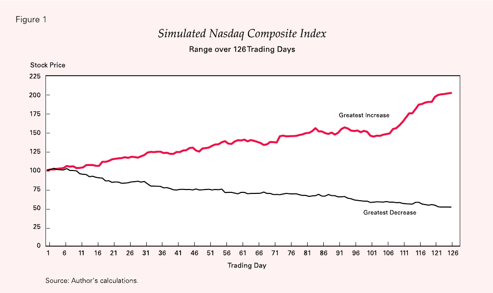
Figure 1 shows the simulated price paths with the

greatest increase and the greatest decrease for the most

volatile index, the Nasdaq Composite. The path with

the greatest increase had a doubling of price, while the

path with the greatest decrease showed smaller

volatility and a halving of price. A more detailed

description of this process is available in Box 3.

The third step was to form the four replicating

portfolios discussed above: a fully levered purchase of

the index, a futures contract, simultaneous purchase of

an index call option and sale of an index put option,

and simultaneous purchase of an index futures call

option and sale of an index futures put option. The ini-

tial and maintenance margin requirements as reported

in Tables 2 and 3 were then applied to the simulated

values of each of the four portfolios, and the margin

deficiency for each day was calculated as the actual

equity less the required margin. This was done for

each of the 126 trading days in a repetition and then

repeated for 10,000 repetitions. The result is 10,000 ran-

domly selected trials of 126-trading day margin

requirements.

For the margin deficiency simulations, the initial

and maintenance margin requirements for the stock

index are 50 percent (Regulation T) and 35 percent,

respectively. The latter is the modal maintenance mar-

gin requirement adopted by NASD members in the

late 1990s. The initial margin requirement for stock

index futures is 6.9 percent for the S&P 500, 8.1 percent

for the NASD Composite, and 5.8 percent for the

Russell 2000. These are the CME’s initial margins for

“speculators,” translated from the absolute dollar val-

ues shown in Table 3 to percentages of the initial index

Fortune pgs 31-50 1/6/04 8:21 PM Page 45

46 2003 Issue New England Economic Review

Box 3

Simulating Asset Prices

Our simulations of R, the daily return on a

stock or stock index, begin with econometric esti-

mation of the five parameters (, , , , and ) that

describe the jump-diffusion processes in equations

(1) and (2) of Box 2. Once estimates of  and  are

available, a random number generator is used to

create the standard normal random variable, e, for

each “day,” and the first part of equation (1) in Box

2, that is, the simple diffusion component,  + e, is

calculated.

The jump effect, v, is then calculated by using

the estimate of  in a Poisson distribution to calcu-

late the random number of jumps, x, on each day.

The parameters describing the mean size and vari-

ability of the size of each jump ( and , respective-

ly) are used with a Normal random number genera-

tor to create the size of each of the jumps during a

day. The value of v is calculated using equation (2)

in Box 2, and this is added to the simple diffusion

component of R described above. The result is, for a

single day, a simulated value for R.

This is done for each of the 126 trading days in a

180 calendar-day period. The same five parameter

values are used for each day, but on each day there

are different values of e and v, and hence a different

value of R, because different draws from the ran-

dom number generator s are made. Once this is

done for all 126 trading days, a single price path

(“trial”) has been computed. This exercise is repeat-

ed until 10,000 trials have been completed. The

result is 10,000 paths, each for 126 days, of the rate of

return on the underlying index. This is transformed

to the level of the index simply by multiplying the

previous index level by the current day’s rate of

return, using the formula S

= S

t-1

(1+R

) where R

the simulated index return for the t

day in a trial.

The simulated path of the futures contract on

the underlying stock index is then calculated. Using

the notion of index arbitrage to link spot and

futures prices, the futures price in a contract expir-

ing at the end of 180 calendar days is the spot price

“grown” at the fixed daily rate of interest, denoted

by r; thus, F

= S

(1+r)

180

Call and put option prices for the stock index

are computed using a jump-diffusion variant of the

Black-Scholes option pricing model. For each possi-

ble number of jumps in a day (x = 0, 1, 2,… ) the val-

ues of the call and put options are computed using

Black-Scholes; call them C

, x ) and P

, x),

where S

is the day’s index value and x is a specific

number of jumps. Then the call and put option pre-

miums are computed as a weighted average of

these number-of-jump-specific call and put option

prices, or:





–



/ x!]C

,x), and

x = 0





–



/ x!]P

,x). and

x = 0

The weights are the Poisson distribution proba-

bilities associated with each number of jumps; these

probabilities depend on the parameter , which

measures the average number of jumps on any day.

This gives, for each day in a trial, the simulated

stock index option values. Repeating this for each of

the 126 trading days gives a single price path, and

doing the same thing for all 10,000 trials completes

the computation of 126 days of option prices for

each of 10,000 trials.

The values of call and put options on futures

contracts are computed in the same way. That is, for

each possible number of jumps in a day, the values

, x ) and P

, x) are computed. These are the

call and put option premiums given the day’s

futures price and the number of jumps. The value of

the futures call or put option is also computed as

the weighted average of the number-of-jump-spe-

cific option values, with the weights determined by

the Poisson distribution.

At the end, we have six 126 X 10,000 matrices of

values, one matrix for each of the prices involved:

the index price, its futures price, prices of call and

put options on the index, and prices of call and put

options on the index futures contract. These prices

are then used to calculate the required margin and

actual margin on each “replicating portfolio” on

each day.

A 126 X 10,000 matrix of cash margin calls is

constructed. From this matrix the “final” margin

cost is calculated as the accumulated value at the

end of the 180 calendar days of each margin call,

assuming payment is made at the end of the day on

which the call is issued.

Fortune pgs 31-50 1/6/04 8:21 PM Page 46

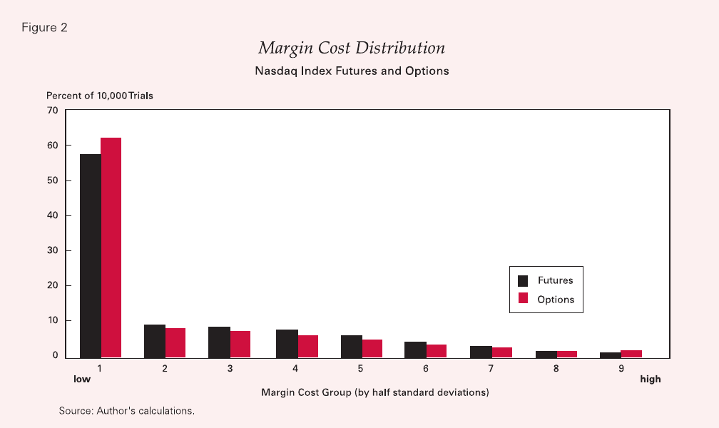
2003 Issue New England Economic Review 47

value in mid-June 2003. Because variation margin is

collected, maintenance margins on index futures con-

tracts are equal to initial margins. The initial margin

requirements for options on the stock index and on its

index futures contracts are those reported in Table 2

for a long call and a short put, both naked: The margin

required on the long call is the initial long call premi-

um; the margin on the short put is the day’s short put

premium plus 15 percent of the index value less the

out-of-money value of the short put option.

In calculating the margin call for each day, we

assumed that if the margin deficiency is negative

(there is excess margin), the trader lets the credit bal-

ance stay in the account rather than withdrawing it

in cash. If the margin deficiency is positive, the trad-

er must make cash payments to satisfy the deficien-

cy. Any prior excess margin can be used to satisfy the

deficiency, but cash must make up any remaining

shortfall. Using these rules, cash margin calls were

constructed for each day and for each repetition.

Each day’s cash payment was then accumulated to

the end of the 180

calendar day at the riskless rate

of interest. The final result is a total cash cost of mar-

gin calls for each of the 10,000 trials. This allows an

assessment of the burden of margin costs across

equity-related instruments and of the potential

effect that these costs have on choices by traders

and investors.

The simulations do not consider some important

aspects of investor choice. Most importantly, we

assume that the initial position is held for the full 180

days. Clearly, investors have the option to exit their

portfolios at any point, and a sequence of dismal days

with margin calls will induce many investors to sell

their positions. But we have not incorporated a model

of exit choice into the simulations, so we assume that

investors hold their positions for the entire period.

Our estimates of margin costs are, therefore, overstat-

ed if the investor exits early. We also do not incorpo-

rate price limits—a prominent feature of futures con-

tracts—into our simulations.

Results

Figure 2 and Table 5 summarize the information

on the distribution of margin costs for each of the four

portfolios. Figure 2 shows the distribution of margin

cost for the Nasdaq Composite as a histogram. The rel-

ative frequency of margin costs in each cost group is

shown for index futures and for index options. Margin

cost groups are defined in terms of standard devia-

tions from the average margin cost for the instrument.

Fortune pgs 31-50 1/6/04 8:21 PM Page 47

48 2003 Issue New England Economic Review

Group 1, the lowest group, consists of final costs

between 0.5 and 1.0 standard deviations below the

mean, group 2 represents observations between the

mean and 0.5 standard deviations below the mean,

group 3 is observations between the mean and 0.5

standard deviations above the mean, and so on. Group

9 is observations more than three standard deviations

above the mean. Note that the margin cost data are

standardized for purposes of exposition, and that the

means (and standard deviations) are different for

futures and options. Expressed as a percent of the ini-

tial underlying index, the mean and standard devia-

tion for Nasdaq futures margin cost are 14.1 percent

and 8.7 percent, respectively; for Nasdaq options, they

are 37.8 percent and 13.5 percent, respectively. Thus,

margin costs are higher and more variable for index

options than for index futures.

Figure 2 shows that the fre-

quency distributions of margin

costs are similar for futures and

options. About 58 percent of

futures observations and 62 per-

cent of options observations are

in the lowest-cost group. About

2 percent of observations are in

the highest group—over three

standard deviations above the

mean margin cost. The lower

boundary of this highest group

is about 40 percent for futures

and 78 percent for options.

Table 5 shows the distribu-

tion of the absolute dollars of

margin cost, expressed as a per-

centage of the initial stock index

(assumed to be $100). Thus, for

the Nasdaq Composite, the 99

percentile of margin costs for the

stock purchase strategy is 57.8

percent of the initial index level,

or $57.80 per $100 of initial

value.

The median margin cost is

highest for the stock purchase

strategy, lowest for the futures

contract, and intermediate for

the index option and index

futures option strategies. Thus,

for the S&P 500, the median cost

is 51.3 percent for the stock

index, 7.1 percent for the futures

index, and about 26 percent for

the option contracts. Stock index derivatives are a

lower-cost way of getting the returns on the index,

with the margin cost advantage being particularly

great for futures index contracts. This is true for all

three indexes, and it is true for all indexes up to

approximately the 90

percentile. In short, there is at

least a 90 percent probability that derivatives will

carry lower margin costs than outright purchase.

If the advantages are so great, why don’t all

traders use derivatives? One reason is that there are

non-margin cost differences among the three strate-

gies. For example, price limits in futures contracts

make them less liquid and, therefore, less desirable.

But another reason is that in particularly bad times, the

margin costs jump more sharply for derivatives than

for outright purchase of the stock index. Consider the

Nasdaq Composite. There is a one percent chance that

Table 5

Distribution of Cost of Margin Calls

Selected Common Stock Price Indexes

Percent of Initial Stock Index

Security Class

Stock Stock Futures

Index Index Futures Options Options

S&P 500

Maximum 59.5% 43.6% 88.0% 88.5%

Percentile 51.3 30.9 64.3 64.8

Percentile 51.3 24.4 52.2 52.8

Percentile 51.3 13.8 33.3 33.7

Percentile 51.3 7.1 25.7 26.0

Percentile 51.3 7.1 25.6 26.0

Minimum 51.3 7.1 25.1 26.0

Nasdaq Composite

Maximum 69.1% 59.7% 119.9% 120.4%

Percentile 57.8 42.2 85.0 85.5

Percentile 52.1 33.2 68.5 69.0

Percentile 51.3 18.3 41.6 42.1

Percentile 51.3 8.4 30.1 30.5

Percentile 51.3 8.3 30.1 30.5

Minimum 51.3 8.3 30.1 30.5

Russell 2000

Maximum 61.5% 45.5% 93.8% 94.3%

Percentile 51.5 30.1 64.5 65.1

Percentile 51.3 23.2 51.9 52.4

Percentile 51.3 12.6 32.8 33.3

Percentile 51.3 6.0 25.2 25.5

Minimum 51.3 6.0 25.2 25.5

The cost of margin calls is computed as follows: The margin call on each day is calculated and

“grown” to the 180

calendar day at the riskless rate of interest. These daily cumulative costs

are then summed to obtain the aggregate cost of margin calls. Results are expressed as a

percent of the initial value of the stock index (assumed to be $100).

Fortune pgs 31-50 1/6/04 8:21 PM Page 48

2003 Issue New England Economic Review 49

the futures index margin costs will rise to 42.2 percent

or more—still below the 57.8 percent margin cost asso-

ciated with outright purchase, but well above the 8.4

percent median margin cost. And the option contracts

fare even worse in bad times: The 99

percentile for

option margin costs is about 85 percent—well above

the stock index’s 57.8 percent and the futures index’s

42.2 percent.

Thus, an investor’s choice of which strategy to

adopt is not a simple matter of considering the average

level of margin costs. It also depends on the sensitivity

of margin costs to changes in the underlying stock

index and on the investor’s taste for risk. Risk-tolerant

investors might prefer the use of derivatives because

the low average cost compensates them for the rare

experience of high margin costs. Investors who do not

tolerate risk well might prefer the strategy of outright

purchase.

V. Summary and Conclusions

Innovations in financial instruments have broad-

ened the ways that investors can achieve their desired

risk and return characteristics. This study shows that,

absent any cash costs from trading (bid-ask spreads,

commissions and fees, cash payment for margin

requirements), the following are identical ways to

invest in the S&P 500 index: a fully leveraged purchase

of a “Spider”; taking a long position on a futures con-

tract on the S&P 500 index; buying a call option on the

S&P 500 and simultaneously selling a put option, both

at a specific price; and buying a futures call option

while simultaneously selling a futures put option,

again at a specific strike price. While stock index

instruments are the focus of the study, the same princi-

ples apply to investing in individual stocks or their

derivatives.

Why would an investor prefer one strategy over

another? The reason must lie in differences in costs, or in

legal and regulatory features that make one market dif-

ferent from another or that inhibit entry into one or more

markets. This study focuses on one aspect of the deci-

sion—costs related to margin requirements. Regulations

at the federal, exchange, house, and clearinghouse levels

require investors to put up cash or acceptable securities

to meet margin (equity) requirements.

The study describes the current margin require-

ments on stocks, stock options, futures contracts, and

futures contract options. It notes that one of the impor-

tant differences between margin requirements on stocks

and on stock derivatives is that maintenance margin

requirements on derivatives are set at the initial margin

requirement level, with variation margin required to

maintain the equality. In contrast, requirements on

stocks are set at the time of purchase but do not change

after purchase unless prices decline sufficiently to

induce maintenance margin calls. Thus, margin require-

ments on derivatives should be more variable over the

holding period than requirements on stock.

This hypothesis is supported by a stochastic simu-

lation of the prices of three stock indexes: the Nasdaq

Composite, the S&P 500, and the Russell 2000. Margin

requirements for these indexes and for index-related

derivatives are calculated, and the costs of the cash

margin calls are computed. The primary conclusion is

that the average (median) cost of margin requirements

for index futures contracts is far less than the average

cost of stock index margin requirements, while the

average cost of margin requirements on stock index

options is between that for stock indexes and index

futures but closer to the former. Thus, an investor

focusing on average experience would have a strong

incentive to hold futures contracts and a moderate

preference for options contracts over outright pur-

chase of a stock index. The same ranking would, of

course, apply to holding individual stocks.

However, the margin requirement costs of futures

and options are highly variable. While the futures con-

tract margin cost is always less than the almost fixed

margin cost of holding the index itself, the futures

investor can experience dramatic fluctuations in mar-

gin costs. The same is true for options contracts, where

investors have a small chance of incurring greater

margin costs than in an outright purchase. Investors

who forego the fixed costs of stock ownership accept

the highly variable costs of derivatives, exposing

themselves to a small chance of facing liquidity prob-

lems that force an untimely exit from positions. Thus,

the ranking of strategy preferences will depend on

investors’ preferences: Risk-tolerant investors, who

focus on average costs rather than cost variability, will

choose futures contracts; less risk-tolerant investors

have reason to choose options contracts or outright

purchase.

The study shows that the structure of margin

costs is rather complex, and that it is difficult to deter-

mine whether the playing field is level because not all

investors are identical. The conventional view that

margin costs provide a clear incentive to use deriva-

tives—particularly futures contracts—ignores the dif-

ferences in the fixed vs. variable cost structure of mar-

gin costs: Investors are sorted into different markets,

allowing all instruments to be financially viable.

Fortune pgs 31-50 1/6/04 8:21 PM Page 49

50 2003 Issue New England Economic Review

References

Edwards, Franklin R. 1983. “The Clearing Association in Futures

Markets: Guarantor and Regulator.” Journal of Futures Markets

3(4): 369–392.

Estrella, Arturo. 1988. “Consistent Margin Requirements: Are They

Feasible?” Federal Reserve Bank of New York. FRBNY Quarterly

Review. Summer 13(2): 61–79.

Figlewski, Stephen. 1984. “Margins and Market Integrity: Margin

Setting for Stock Index Futures and Options.” Journal of Futures

Markets 4(3): 385–416.

Fortune, Peter. 1999. “Are Stock Returns Different Over Weekends?

A Jump Diffusion Analysis of the ‘Weekend Effect’.” Federal

Reserve Bank of Boston. New England Economic Review.

September/October: 3–19.

___________. 2000. “Margin Requirements, Margin Loans, and

Margin Rates: Practice and Principles.” Federal Reserve Bank of

Boston. New England Economic Review. September/October: 19–44.

___________. 2001. “Margin Lending and Stock Market Volatility.”

Federal Reserve Bank of Boston. New England Economic Review.

Fourth Quarter: 3–25.

___________. 2002. “Security Loans at Banks and Nonbanks:

Regulation U.” Federal Reserve Bank of Boston. New England

Economic Review. Fourth Quarter: 19–40.

Gay, Gerald D., William C. Hunter, and Robert W. Kolb. 1986. “A

Comparative Analysis of Futures Contract Margins.” Journal of

Futures Markets 6(2): 307–324.

Kupiec, Paul H. 1994. “The Performance of S&P 500 Futures Product

Margins under the SPAN Margining System.” Journal of Futures

Markets 14(7): 789–811.

Minehan, Cathy E. and Katerina Simons. 1995. “Managing Risk in

the ‘90s: What Should You Be Asking about Derivatives?” Federal

Reserve Bank of Boston. New England Economic Review.

September/October: 3–25.

Ritchken, Peter. 1987. Options: Theory, Strategy, and Applications.

Glenview, IL: Scott, Foresman and Company.

Rutz, Roger. 1989. “Clearance, Payment and Settlement Systems in

the Futures, Options and Stock Markets.” Board of Trade Clearing

Corporation, Chicago, IL. mimeo.

Sofianos, George. 1988. “Margin Requirements on Equity

Instruments.” Federal Reserve Bank of New York. FRBNY

Quarterly Review. Summer 13(2): 47–60.

Fortune pgs 31-50 1/6/04 8:21 PM Page 50

2003 Issue New England Economic Review 51

Fortune pgs 31-50 1/6/04 8:21 PM Page 51